measure and attribute stratified heterogeneity with software |
||||||||||||||||||||||||||||||
|
||||||||||||||||||||||||||||||
Articles
using Geodetector [Numbered]
Updated on 30
September 2023 4. Download of the software, with example
datasets |
||||||||||||||||||||||||||||||
1.
Introduction
Spatial Stratified Heterogeneity (SSH) is a phenomena that the within strata are more similar than the between strata. Examples of this include landuse types and climate zones in spatial data, seasons and years in time series, occupations, age groups, incomes strata. SSH occurs in all scales from universe to DNA, and has been studied since Aristotle time. Geodetector, or Geographical
Detector, is a statistical tool to measure SSH and to make attributions for or
by SSH (Fig. 1): (1) Measure and identity SSH among data; (2) Test the coupling between two variables Y and X without assuming linearity of the association and with clear
physical meanings; and (3) Investigate the general interaction between two explanatory
variables X1 and X2 and a response variable Y, without any specific form of
interaction such as the assumed product in econometrics (Fig. 2). Each of the above tasks can be accomplished
using the Geodetector q-statistic:
Fig. 1. Principle of Geodetector q-statistic
(Wang et
al 2016) (The bottom map, the
color indicates the values of a population Y. The top map, the population Y is composed of L
strata (h = 1, 2, …, L); the terms “stratification” and
“partition” are equivalent, can be either classification or zonation. Between
the two maps is the equation q(Y|{h}),
in which the numerator is the summation of the within strata variance and the
denominator is the pooled variance; N
and s2 stand for the number
of units and the variance of Y in a
study area, respectively. [(N-L)q]/[(L-1)(1-q)] ~ F(L-1, N-L, g), where g is a non central parameter) . The strata of Y (red
polygons in Fig.1) are a partition
of Y, either by Y itself or by an explanatory variable
X. X is a categorical variable or should be stratified if it is a
numerical variable. The number of strata L
might be 2-10 or more, according to prior knowledge or a classification
algorithm. The “spatial” in “spatial stratified heterogeneity”
can be either spatial in geoscience or in a broad mathermatical sense such as
time and any attributes. Interpretation of Geodetector q-statistic (Fig.1). The value of q is strictly within [0, 1]. (1) If Y is stratified by Y
itself, then a q-statistic of 0
indicates that Y is absent of
spatial stratified heterogeneity; a q-statistic
of 1 indicates that Y is perfectly
spatially stratified heterogenous; and a q-statistic
of 100q% measures the degree of
spatial stratified heterogeneity of Y. (2) If Y is stratified by an explanatory variable X, then a q-statistic
of 0 indicates that there is no coupling between Y and X; a q-statistic of 1 indicates that Y is completely determined by X; and X explains 100q% of Y. Please note that the q-statistic measures the association
between X and Y without assuming the linearity between X and Y. Geodetector q-statistic
can be used to understand spatial confounding, sample bias and overfitting. (1)
Confounding can occur if a model is applied to a (spatial)
stratified heterogeneneous population, leading to a misleading interpretation
and statistical insignificance of the model outcome. This problem can be
avoided by identifying SSH (by Geodetector q statistic) then modelling in the strata, separately. (2)
A sample would be biased if a population is
(spatial) stratified heterogeneous and the sample do not cover all strata.
The problem can be solved by identifing (spatial) stratified heterogeneity
(using Geodetector q statistic)
then applying bias remedy models such as Heckman regression and Bshade
method. (3)
Local models aim to overcome heterogeneity but
often suffer from overfitting and too many parameters to interpret. These
problems can be avoided by modelling in strata or stratifying the outputs of
a local model then interpreting the stratified parameters. Functions of Geodetector: (1)
The risk detector maps response variable Y in strata according to X; (2)
The factor detector q-statistic
measures the degree of spatial stratified heterogeneity of a variable Y if Y is stratified by itself; and the determinant power of an
explanatory variable X on Y if Y is stratified by X; (3)
The ecological detector identifies the difference in the impacts
between two explanatory variables X1
and X2; (4)
The interaction detector reveals whether the risk factors X1 and X2 (and more X, if applicable) have an interactive
influence on a response variable Y
(Fig.2). 
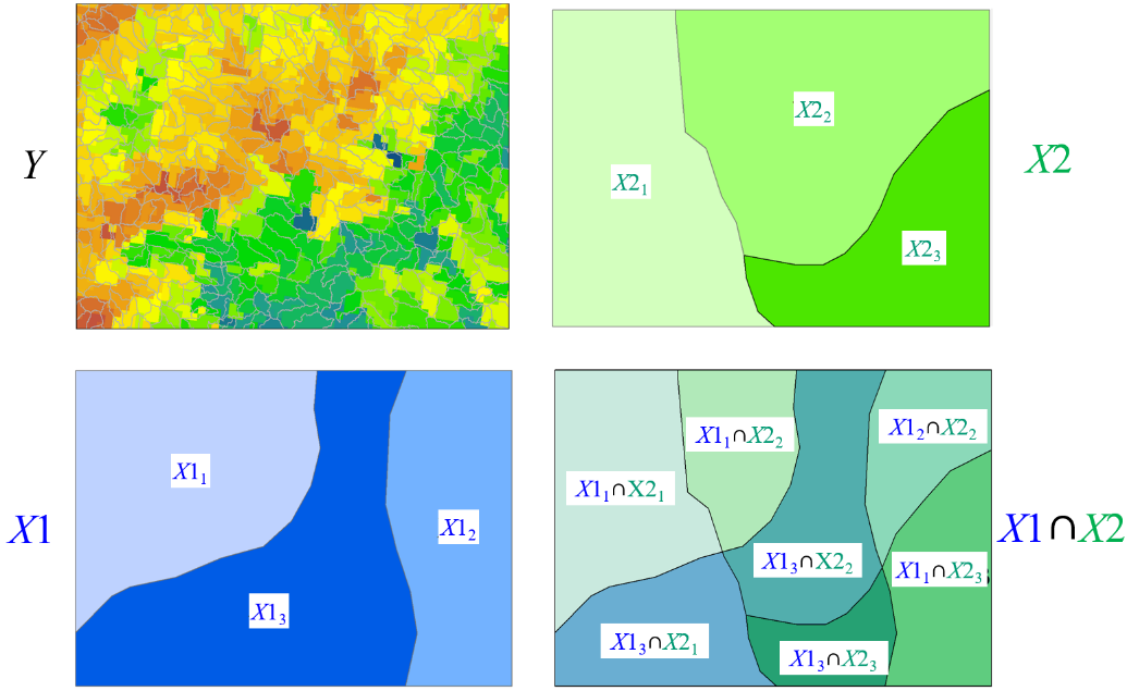
Fig.
2. The General
interaction between explanatory variables X1 and X2
impacting on a response variable Y:
q(Y|X1 |
2.
Tutorial
The Geodetector software was developed using
Excel and R, respectively. The tools are free of charge, freely downloadable,
and easy to use, and were designed without any GIS plug-in components and
with “one click” execution. Users can run the following demo, then simply
replace the demo data in the software using your own data, click Run and get
results ! We henceforth describe Excel Geodetector software. R users can
download the R Geodetector software in the following section “Download of Geodetector Software and
Example Datasets”. As a demo, neural-tube birth defects (NTD) Y and suspected risk factors or their proxies Xs in villages are provided, including
data for the health effect layers “NTD prevalence” and environmental factor
layers, “elevation”, “soil type”, and “watershed”. Their field names are
defined as Y and X1, X2, X3 respectively. Step 1. Download the software and input your
data in Excel (1) Download the Excel
Geodetector software (In the following section “Software and Examples Data
Download”), one click to download any one of the three Examples, unzip the
downloaded file, you will find an Excel file (this is Geodetector software
with an Example dataset!) and double click the Excel file, Fig. 3 and Fig. 5 appear. Fig. 3
is the format of the input data for the Geodetector: each row denotes a
sample unit (e.g. a village); the 1st column record the response
variable Y; the 2nd and
following columns denote partitions of Y
or factors X, the latter were
partitioned according to the similarity within strata. (2) Input your data into
the Excel Geodetector software in the format of Fig. 3. Then go to Step 2. Fig. 3. Input data in Excel and the execution interface (Note: Y should be numerical; X MUST be categorical, e.g. landuse types,
seasons. If X is numerical, it
should be transformed into a categorical variable, e.g. GDP per capita is
stratified into 5 strata. At lease three sample units in each of the strata
are required) (3)
If your data is in GIS format, as shown in Fig. 4, you can use QGIS directly in Section 4, or you can transform the GIS data into Excel data as
shown in Fig. 3. Fig. 4. Data in GIS format Step 2. Run Geodetector
software Only one operation interface was designed (Fig. 5). The function of the “Read
Data” button is to load data; thus, when the button is clicked, all variables
are listed in the “variables” list box. Then, disease and partition of Y or environmental factor variables
are selected into their corresponding list boxes Y and X on the right of the
interface. Finally, Geodetector is executed by clicking the “Run” button. Fig. 5. User interface for Geodetector back to the top ||
|
3.
Output
Geodetector outputs
results from the risk detector, factor detector, ecological detector, and
interaction detector in four Excel spreadsheets (Fig. 6). Fig. 6. Interface
for Geodetector results In the “Risk detector”
sheet (Fig. 7), result information
for each environmental risk factor is presented in two tables. The first
table gives the average disease incidence in each stratum of a
risk factor, the name of which is written at the top left of the table. The second
table gives the statistically significant difference in the average disease
incidence between two strata; if there is a significant difference, the
corresponding value is “Y”, else it is “N”. Fig. 7. Results of risk detector The
Fig. 8 shows the output format of
the q values for each environmental
risk factor, as given in the “Factor detector” sheet. The table header gives
the names of the environmental risk factors X(X1, X2, …, Xn), while the associated q
values and their corresponding p
values are presented in the row below. Fig. 8. Results of factor detector In the “Ecological
detector” sheet (Fig. 9), results of the statistically
significant differences between two environmental risk factors are presented.
If Y(X1) (risk factor names in row) was significantly
bigger than Y(X2) (risk factor names in column), the associated
value is “Y”, while “N” expresses the opposite meaning. Fig. 9. Results of ecological detector The format of the results for the interaction detector is shown in Fig. 10. “Interaction relationships” below the table represent the interaction relationship for the two factors. The relationship is defined in a coordinate axis. It has 5 intervals, including “(-∞,min( |